Formula

curabaysevket · September 4, 2024, 1:35pm

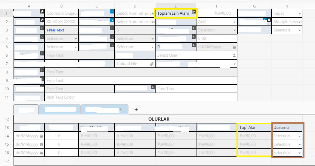
I want to create a formula in Cell E1. I want to add the G13 subtable values of the (Aktif) (Taahhüt) and (S.Teslimi) selected in the H13 Subtable. I would be happy if you could help.

ting · September 6, 2024, 3:05am

Hi,

To achieve what you’re aiming for in cell E1, you can use the SUMIF() formula to sum the values in G13 that meet the conditions in H13. Here’s the formula you can apply:

SUMIF(H13, “Aktif”, G13) + SUMIF(H13, “Taahhüt”, G13) + SUMIF(H13, “S.Teslimi”, G13)

This formula will add the G13 values that correspond to “Aktif”, “Taahhüt”, and “S.Teslimi” in the H13 subtable.

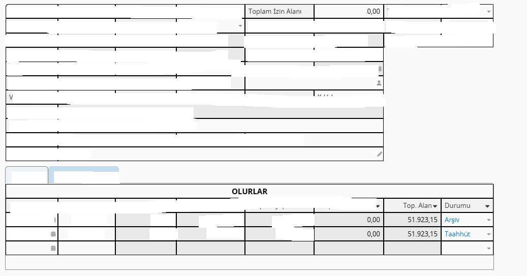
curabaysevket · September 6, 2024, 7:00am

thanks for answer but I get a warning

Your formula contains an error. Please make sure that all parentheses are part of a matching pair, and whether you have entered all required arguments.

ting · September 6, 2024, 7:37am

Hi,

I tested it on my sheet, and it seems to work fine. Do you happen to have a screenshot ? It could help check if there are any incorrect symbols in the formula.

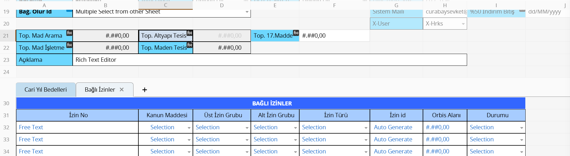
curabaysevket · September 18, 2024, 9:40pm

A21 hücresinde bir formül oluşturmak istiyorum. alt tablosunda I31 seçili olan (Aktif) (Taahhüt) ve (S.Teslimi) değerlerinin ve E31 de (Maden Arama) değerlerinin toplanmasını istiyorum.
C21 hücresinde bir formül oluşturmak istiyorum. alt tablosunda I31 seçili olan (Aktif) (Taahhüt) ve (S.Teslimi) değerlerinin ve E31 de (Altyapı Tesis) değerlerinin toplanmasını istiyorum.
A22 hücresinde bir formül oluşturmak istiyorum. alt tablosunda I31 seçili olan (Aktif) (Taahhüt) ve (S.Teslimi) değerlerinin ve E31 de (Maden İşletme) değerlerinin toplanmasını istiyorum.

ting · September 20, 2024, 7:53am

Hi,

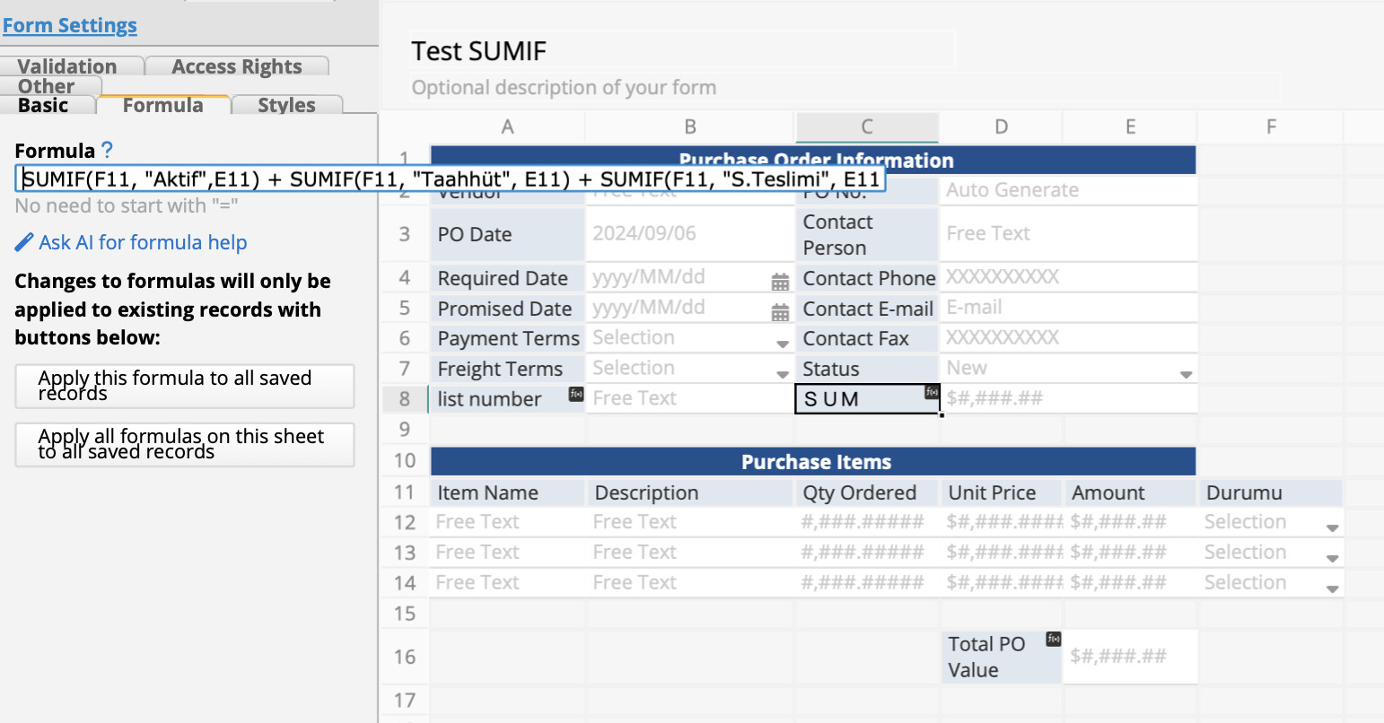
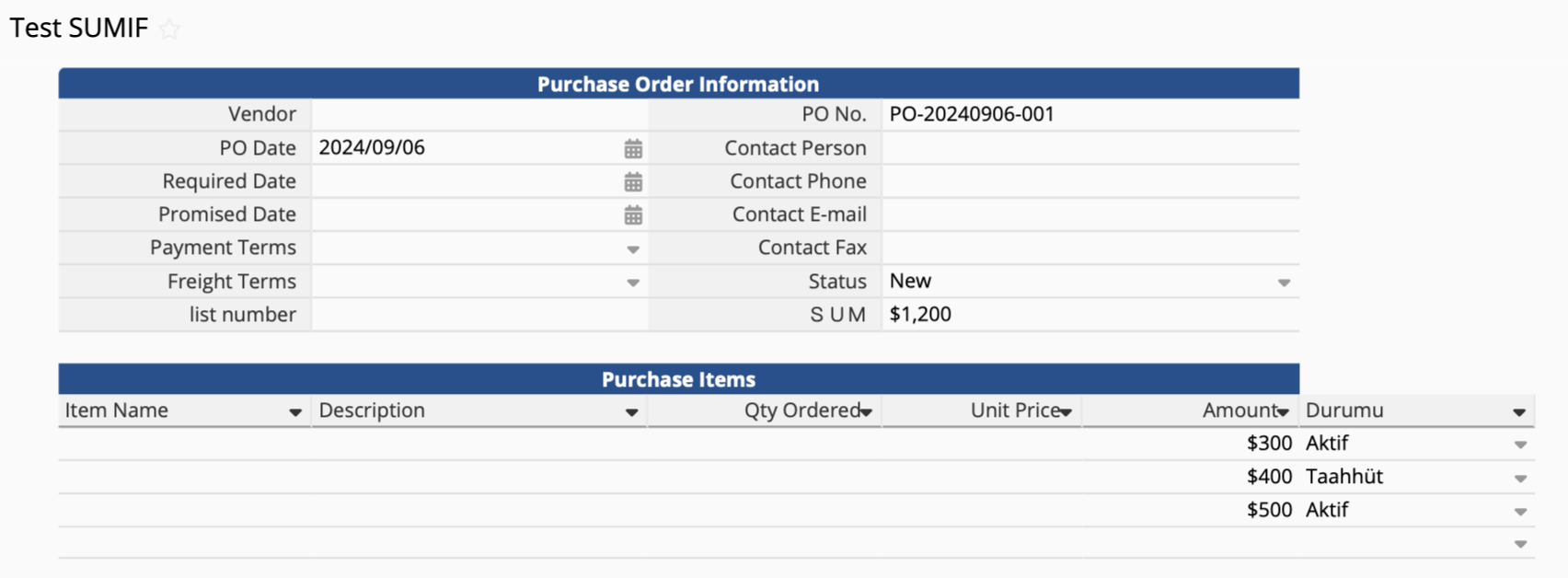
Thank you so much for sharing the screenshot! Could you please provide a screenshot of the formula? Just like to check for any special characters or settings that might be causing the issue. Since the formula I shared earlier works perfectly on my end.

Thank you!

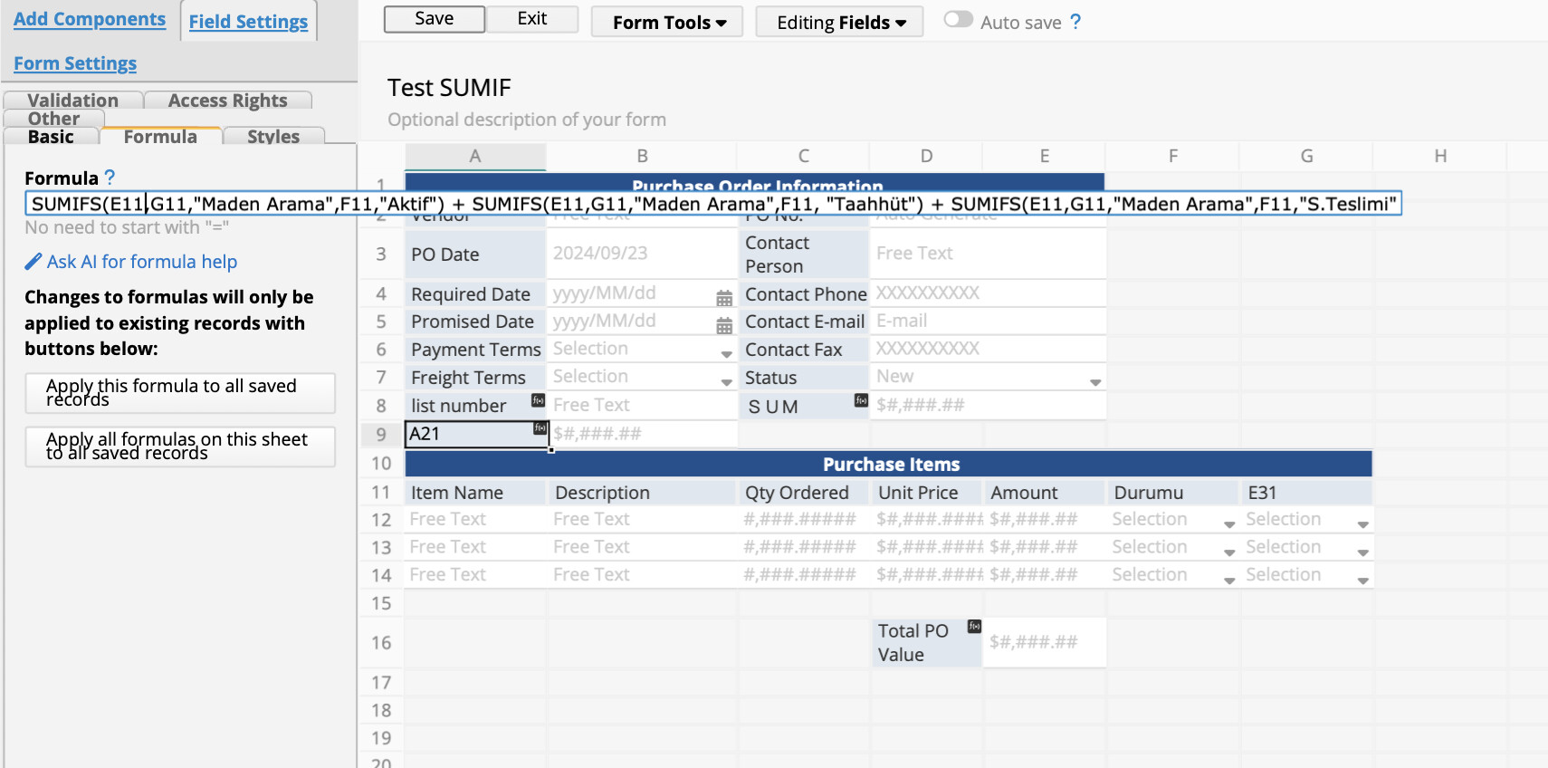
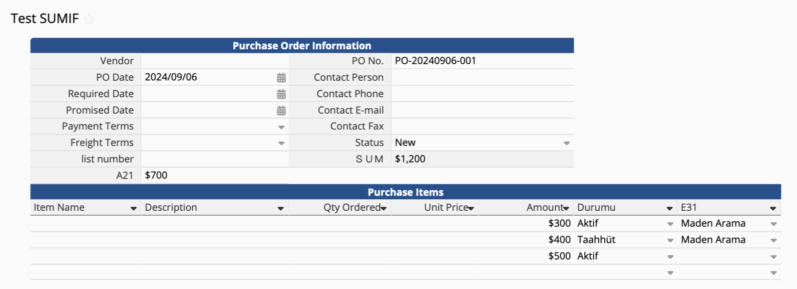
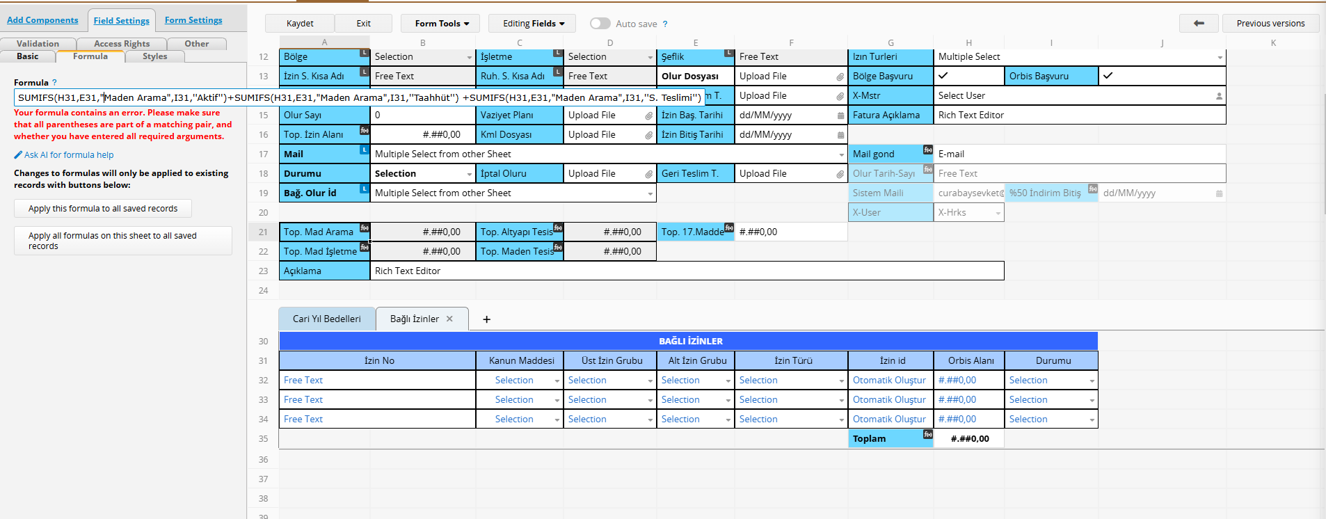
curabaysevket · September 20, 2024, 10:15am

The previous formula worked, now I added one more condition but I could not create the formula again. I would appreciate if you can help. The screenshot I mentioned and the terms at the bottom I shared in a previous screenshot and at the bottom.

ting · September 23, 2024, 10:08am

Hi,

If you want to perform a conditional sum using more than one criterion, you may use the SUMIFS() formula.

curabaysevket · September 23, 2024, 12:08pm

Thank you for your interest. But it gives me an error about the formula.

ting · September 26, 2024, 6:36am

Hi,

Thank you so much for providing the screenshot! However, it’s a bit difficult to fully understand the database design and formula issue just from the image. Could you kindly contact us via the upper right corner of the database “Need Help?” > “Support Ticket” so we can check the exact sheet and better identify the problem? Thanks again for your help!